Transhipment Problem

This example is taken from the MOOC MITx: CTL.SC2x (edX plateform). You can check the MOOC for more information about mathematic programming and the implementation with excel.

In this post, I propose an implementation using Gurobi Python environment. Here a transhipment constraint is added to the initial problem (look at older posts on the blog).

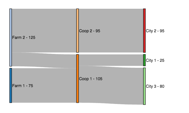
Following Sankey diagram represents the solution to this problem.

Input data

\(S_{i} : \text{production of tomatoes from each Farm (in tons)} \qquad \forall i \in S\) \(D_{j} : \text{demand from each City (in tons)} \qquad \forall j \in D\) \(c_{i,j} : \text{transportation cost between Farm i and City j (€/ton)} \qquad \forall i,j\)

Decision variables

\(x_{i,j} : \text{flow on arc from i to j} \qquad \forall i,j\)

Objective

Minimisation of the transportation cost

\[\min \sum\limits_{i \in{S}}\sum\limits_{j\in{D}} x_{i,j} * c_{i,j}\]

Supply constraint

Production of each farm cannot exceed the sum of the deliveries to all the cities.

\[\sum\limits_{j\in{D}} x_{i,j} \leq S_{i} \qquad \forall i \in S\]

Demand constraint

Demand of each city must be satisfied : one city can be delivered by two farms.

\[\sum\limits_{i\in{S}} x_{i,j} \geq D_{j} \qquad \forall j \in D\]

Transhipment constraint

Amount of tomatoes arriving at one cooperative must be equal to the amout of tomatoes going out.

\[\sum\limits_{i\in{S}}{ x_{i,j}} = \sum\limits_{i\in{S}} x_{j,i} \qquad \forall j \notin S, \notin D\]

Non negativity constraint

\[x_{i,j} \geq 0 \qquad \ \forall i,j\]

---

Python implementation

from gurobipy import *


farms = ["Farm1", "Farm2"]
cities = ["City1", "City2", "City3"]
coops = ["Coop1", "Coop2"]

supply = { "Farm1" : 100,
           "Farm2" : 125}

demand = { "City1" : 25,
           "City2" : 95,
           "City3" : 80}

arcs, cost_tuple = multidict({ ("Farm1", "Coop1") : 190,
                               ("Farm1", "Coop2") : 210,
                               ("Farm2", "Coop1") : 185,
                               ("Farm2", "Coop2") : 105,
                               ("Coop1", "City1") : 175,
                               ("Coop1", "City2") : 180,
                               ("Coop1", "City3") : 165,
                               ("Coop2", "City1") : 235,
                               ("Coop2", "City2") : 130,
                               ("Coop2", "City3") : 145})

m = Model("transhipment_pb")

# Decision variables
flow = m.addVars(arcs, obj=cost_tuple, name="flow")

# Supply constraint
supply_constr = m.addConstrs((flow.sum(farm, "*")
                              <= supply[farm] for farm in farms), 
                              name="supply_constraint")

# Demand constraint
demand_constr = m.addConstrs((flow.sum("*", city)
                             >= demand[city] for city in cities),
                             name="supply_constraint")

# Transhipment constraint
tranship_constr = m.addConstrs((flow.sum("*", coop) 
                                == flow.sum(coop, "*") 
                                for coop in coops),
                                name="transhipment_constraint")

m.optimize()

Here you can see the benefits of the multidict object (from Gurobi). In one declaration, I get arcs dictionnary of all the possible arcs and cost_tuple dictionnary of the associated costs.

The dict arcs allows me to create all the decision variables needed.

Total cost of the solution minimizing cost is 56 700 €.

for c in m.getConstrs():
    print(c.ConstrName, c.slack)

>>> supply_constraint[Farm1] 25.0
>>> supply_constraint[Farm2] 0.0
>>> supply_constraint[City1] 0.0
>>> supply_constraint[City2] 0.0
>>> supply_constraint[City3] 0.0
>>> transhipment_constraint[Coop1] 0.0
>>> transhipment_constraint[Coop2] 0.0

The farm 1 still has 25 tons of unsold tomatoes.